Chapter 11
Table of Contents
Data
Alternatively, individual files can be found in the Data section.
Code from chapter
'''
A quick test of the accuracty of linear and cubic spline interpolation

    Written by: myself (email@domain.com)
     Changelog: 240606 - v1.0.0 - initial version
'''
import numpy as np
import scipy.interpolate as spi

# Define a function that returns the y-values for a Gaussian function
def Gaussian(x, A, x0, sigma):
    return A * np.exp(-1 * (x - x0)**2 / (2 * sigma**2))

# Define the parameters of the Gaussian
A = 1
x0 = 0
sigma = 2

# Create the x- and y-values for the fake data
x_data = np.linspace(-5, 5, 8)
y_data = Gaussian(x_data, A, x0, sigma)

# Create the x- and (exact) y-values for the points at which we would like interpolation
x_interp = np.linspace(-5, 5, 1000)
y_interp_exact = Gaussian(x_interp, A, x0, sigma)

# Do the interpolation.  First we will do a linear interpolation
y_interp_linear = np.interp(x_interp, x_data, y_data)

# Do the cubic spline interpolation - first create the cubic spline object
cs = spi.CubicSpline(x_data, y_data)

# Now generate the array of interpolated points using the cubic spline object
y_interp_cubic = cs(x_interp)

# Compute and print the RMSE
print(f"Linear Interpolation RMSE: {np.sqrt(np.sum((y_interp_linear - y_interp_exact)**2)):4.2f}")
print(f" Cubic Interpolation RMSE: {np.sqrt(np.sum((y_interp_cubic - y_interp_exact)**2)):4.2f}")
'''
Produce an interpolated 785 nm raman spectrum with data points that
match an old 532 nm spectrum
Requires: one 532 nm and one 785 nm Raman spectrum
Written by: Chris Johnson and Ben Lear (authors@codechembook.com)
v1.0.0 - 250304 - initial version
'''
import numpy as np
from plotly.subplots import make_subplots
from codechembook.quickTools import quickSelectFolder, quickPopupMessage
from codechembook.symbols.chem import wavenumber as wn
# Scaling factor for 532 data
scale_532 = 2.95
# Get the folder containing the files to process
quickPopupMessage(message = 'Select the folder with the Raman spectra.')
folder_name = quickSelectFolder()
# Read the data: 785 is the new data that has a contaminant, 532 is the old data
x532, y532 = np.genfromtxt(folder_name/'oldNPs.csv', delimiter = ',',
skip_header = 2, unpack = True)
x785, y785 = np.genfromtxt(folder_name/'newNPs.csv', delimiter = ',',
skip_header = 2, unpack = True)
# Interpolate to the 532 spectrum because 785 has the larger span of x points
y785_interp = np.interp(x532, x785, y785)
# Normalize the 532 data and subtract it from the 785 data
y_delta = y785_interp - scale_532 * y532
# Plot the 785 spectrum, the 532 spectrum, and the difference spectrum
fig = make_subplots(2, 1)
fig.add_scatter(x = x532, y = y785_interp, name = '785 nm', row = 1, col = 1)
fig.add_scatter(x = x532, y = scale_532 * y532, name = '532 nm', row=1, col=1)
fig.add_scatter(x = x532, y = y_delta, name = 'Subtracted', showlegend = False, row = 2, col = 1)
fig.update_xaxes(title = f'wavenumber /{wn}')
fig.update_yaxes(title = 'intensity')
fig.update_layout(template = 'simple_white', font_size = 18, width = 3 * 300,
height = 3 * 300, margin = dict(b = 10, t = 30, l = 10, r = 10))
fig.show('png')
fig.write_image('raman.png')Solutions to Exercises
Targeted exercises
Implementing linear interpolation using numpy.interp
Exercise 1
Consider a Gaussian distribution with $x_0 = 0$, $\sigma = 2$, and amplitude of 1.
- Create 1000 $x$-values between -10 and 10, and use this to create y-values with the above Gaussian parameters. This will represent the ’true’ Guassian shape.
- Repeat the above, but with 5, 6, 7, 8, 9, 10, 11, 12 points, each from -10 and 10. These will represent sparsely sampled points.
- For each set of points generated in the second step, perform a linear interpolation using
numpy.interp(). This accepts three positional arguments: an array of $x$-values you wisht to generate interpolated points for, the original $x$-values, and the original $y$ values used for interpolation. - Make a Plotly plot holding a separate subplot for each of the eight sparse arrays. On this plot, have the ’true’ Gaussian shape, the sparsely sampled points, and the interpolated values.
- Comment on how the interpolation improves with sample points.
- Comment on what regions of the Gaussian seem to be reproduced well, and which are not.
import numpy as np
from plotly.subplots import make_subplots
def gaussian(x, x0, sigma, amplitude):
return amplitude * np.exp(-((x - x0) ** 2) / (2 * sigma**2))
fig = make_subplots(rows = 8, cols = 1)
ultra_fine_x = np.linspace(-10,10,1000)
ultra_fine_y = gaussian(ultra_fine_x, x0=0, sigma=2, amplitude=1)
for i, n in enumerate(range(5, 13)):
fig.add_scatter(x = ultra_fine_x, y = ultra_fine_y, line = dict(color = "grey", width = 10),
showlegend = False,
row = i+1, col = 1)
x_coarse = np.linspace(-10, 10, n)
y_coarse = gaussian(x_coarse, x0=0, sigma=2, amplitude=1)
fig.add_scatter(x = x_coarse, y = y_coarse,
mode = "markers",
showlegend = False,
marker = dict(color = "red", size = 15),
row = i+1, col = 1)
lin_y = np.interp(ultra_fine_x, x_coarse, y_coarse)
fig.add_scatter(x = ultra_fine_x, y = lin_y, line = dict(color = "orange"),
showlegend = False,
row = i+1, col = 1)
fig.add_annotation(text = f"n={n}",
showarrow = False,
x = -9, y = 0.2,
row = i+1, col = 1
)
fig.update_layout(template = "simple_white", height = 1200, width = 600)
fig.show("png")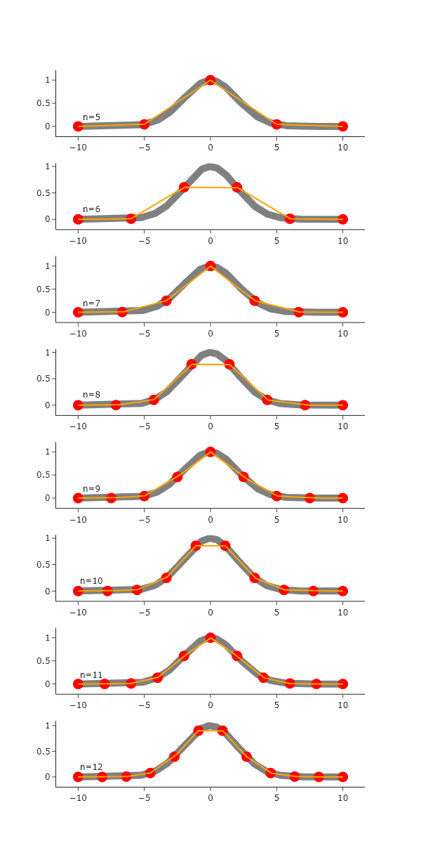 As the number of sparse points increases, the interpolation better agrees with the ’true’ Gaussian, which is expected. The linear interpolation seems to handle regions with out curvature well, but struggles where there is significant curvature.
Implementing cubic spline interpolation using scipy.interpolate.CubicSpline
Exercise 1
Repeat Exercise 0, but use a cubic spline for interpolation.
In addition to answering all parts from Exercise 0, comment on the differences between the results from the linear interpolation, versus the cubic interpolation.
import numpy as np
from plotly.subplots import make_subplots
import scipy.interpolate as spi
def gaussian(x, x0, sigma, amplitude):
return amplitude * np.exp(-((x - x0) ** 2) / (2 * sigma**2))
fig = make_subplots(rows = 8, cols = 1)
ultra_fine_x = np.linspace(-10,10,1000)
ultra_fine_y = gaussian(ultra_fine_x, x0=0, sigma=2, amplitude=1)
for i, n in enumerate(range(5, 13)):
fig.add_scatter(x = ultra_fine_x, y = ultra_fine_y, line = dict(color = "grey", width = 10),
showlegend = False,
row = i+1, col = 1)
x_coarse = np.linspace(-10, 10, n)
y_coarse = gaussian(x_coarse, x0=0, sigma=2, amplitude=1)
fig.add_scatter(x = x_coarse, y = y_coarse,
mode = "markers",
showlegend = False,
marker = dict(color = "red", size = 15),
row = i+1, col = 1)
y_cs = spi.CubicSpline(x_coarse, y_coarse)
y_cubic = y_cs(ultra_fine_x)
fig.add_scatter(x = ultra_fine_x, y = y_cubic, line = dict(color = "orange"),
showlegend = False,
row = i+1, col = 1)
fig.add_annotation(text = f"n={n}",
showarrow = False,
x = -9, y = 0.2,
row = i+1, col = 1
)
fig.update_layout(template = "simple_white", height = 1200, width = 600)
fig.show("png")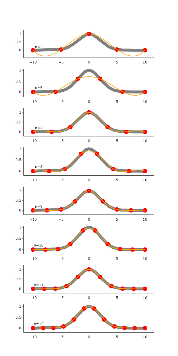 Similar to the linear interpolation, the agreement of the interpolation with the ’true’ Gaussian value increases as the number of sparse points increases. However, the cubic interpolation handles regions of curvature well, and struggles with regions that do not have curvature. The overall agreement also seems to be better for cubic, rather than linear, once the number of points reaches ~9. Thus, as the sampling increases, the cubic interpolation is the clear winner.
Comprehensive
Exercise 2
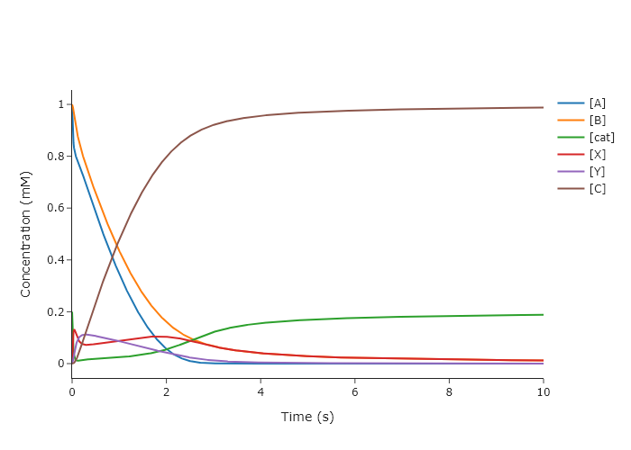
Modify the final code from Chapter 8 to interpolate the kinetic traces so that they have evenly spaced points. Use both linear interpolation and cubic splines. Do you notice any obvious inaccuracies for either method?
'''
A code to numerically solve a reaction mechanism that is irreversible but
has two intermediates using solve_ivp from scipy.integrate
Written by: Ben Lear and Chris Johnson (authors@codechembook.com)
v1.0.0 - 250217 - initial version
v1.0.1 - 250406 - changed so that the spacing along the final t-values is even
'''
import scipy.integrate as spi
from codechembook.quickPlots import quickScatter
import scipy.interpolate as spint
import numpy as np

# First we need to define a function containing our differential rate laws.
def TwoIntermediatesDE(t, y, k):
'''
Differential rate laws for a catalytic reaction with two intermediates:
A + cat ->(k1) X
X + B ->(k2) Y
Y ->(k3) C + cat

REQUIRED PARAMETERS:
t (float):         the cutrent time in the simulation.
                   Not explicitly used but needed by solve_ivp
y (list of float): the current concentration
k (list of float): the rate

RETURNS:
(list of float): rate of change of concentration in the order of y
'''
A, B, cat, X, Y, C = y # unpack concentrations to convenient variables
k1, k2, k3 = k # unpack rates

dAdt   = -k1 * A * cat
dBdt   = -k2 * X * B
dcatdt = -k1 * A * cat + k3 * Y
dXdt   = k1 * A * cat - k2 * X * B
dYdt   = k2 * X * B - k3 * Y
dCdt   = k3 * Y

return [dAdt, dBdt, dcatdt, dXdt, dYdt, dCdt]

# Set up initial conditions and simulation parameters
y0 = [1.0, 1.0, 0.2, 0.0, 0.0, 0.0] # concetrations (mM) [A, B, cat, X, Y, C]
k = [5e1, 1e1, 5e0]                 # rate (1/s)
time = [0, 10]                      # simulation start and end times (s)

# Invoke solve_ivp and store the result object
solution = spi.solve_ivp(TwoIntermediatesDE, time, y0, args = [k])

t_int = np.linspace(0,10,1000) # set up the even spacing along x
y_ints = []
for y in solution.y:
y_cs = spint.CubicSpline(solution.t, y)
y_ints.append(y_cs(t_int))

# Plot the results
quickScatter(x = t_int, # need a list of six identical time axes
         y = y_ints,
         name = ['[A]', '[B]', '[cat]', '[X]', '[Y]', '[C]'],
         xlabel = 'Time (s)',
         ylabel = 'Concentration (mM)',
         output = 'png')